CryoCCD

Simulating Cryo-EM: Cycle-Consistent Predictor–Corrector Diffusion with Biophysical Modeling

A biophysical engine turns protein structures into noise-free micrographs, and the first diffusion model for cryo-EM noise synthesis makes them look like real data.

Transactions on Machine Learning Research (TMLR) 2026

Runmin Jiang1*, Genpei Zhang2*, Yuntian Yang3*, Siqi Wu1, Seonghui Min1, Xi Xiao4, Yizhou Zhao1, Xiao Wang5, Tianyang Wang4, Xingjian Li1, Muyuan Chen6, Min Xu1†

1Carnegie Mellon University · 2University of Wisconsin–Madison · 3Harvard University · 4University of Alabama at Birmingham · 5Oak Ridge National Laboratory · 6Stanford University

*Equal contribution    †Corresponding author

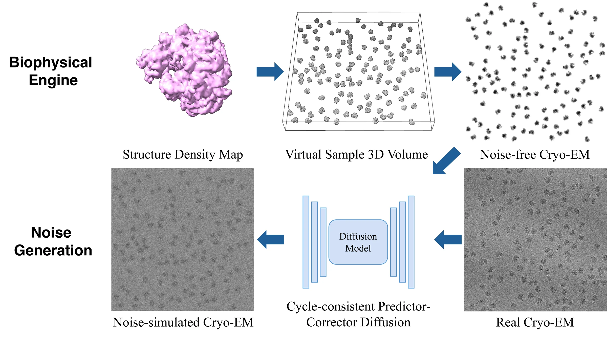
Overview of CryoCCD: a biophysical engine produces noise-free micrographs from density maps; a diffusion model adds realistic noise learned from real cryo-EM.
Simulating cryo-EM with CryoCCD. The biophysical engine builds a virtual specimen from structure density maps and projects it into a noise-free micrograph; a cycle-consistent predictor–corrector diffusion model then synthesizes noise learned from real data (example: EMPIAR-10028, Plasmodium falciparum 80S ribosome).

Abstract

Learning-based cryo-EM tools need more labelled data than exists.

Single-particle cryo-electron microscopy (cryo-EM) has become a cornerstone of structural biology, enabling near-atomic resolution analysis of macromolecules through advanced computational methods. However, the development of cryo-EM processing tools is constrained by the scarcity of high-quality annotated datasets. Synthetic data generation offers a promising alternative, but existing approaches lack thorough biophysical modeling of heterogeneity and fail to reproduce the complex noise observed in real imaging.

To address these limitations, we present CryoCCD, a comprehensive simulator for cryo-EM, unifying versatile biophysical modeling with the first diffusion model for realistic noise generation. The biophysical engine provides multi-functional generation capabilities to capture authentic biological organization, and the diffusion model is enhanced with cycle consistency and predictor–corrector sampling to improve realism and structural fidelity. Extensive experiments demonstrate that CryoCCD generates structurally faithful micrographs, enhances particle picking and pose estimation, as well as achieves superior performance over state-of-the-art baselines, while also generalizing effectively to held-out protein families.
Contributions

What CryoCCD adds

01

A biophysical engine for heterogeneous specimens.

PDB structures and AlphaFold3 predictions are placed into virtual volumes with particle-type-specific distributions, multi-scale meshes and a modeled ice layer, then projected under the weak-phase approximation with a CTF.

02

The first diffusion model for cryo-EM noise.

Unpaired clean-to-real translation with cycle consistency to keep structures intact, mask-guided contrastive learning for fine detail, and a UniPC predictor–corrector sampler for noise fidelity.

03

Gains on realism and on downstream tasks.

Lowest FID and CMMD on six EMPIAR datasets, better particle picking (AUPRC) and pose estimation, and the best scores on four held-out datasets with unseen protein families or imaging conditions.

Method

From atomic structures to realistic micrographs

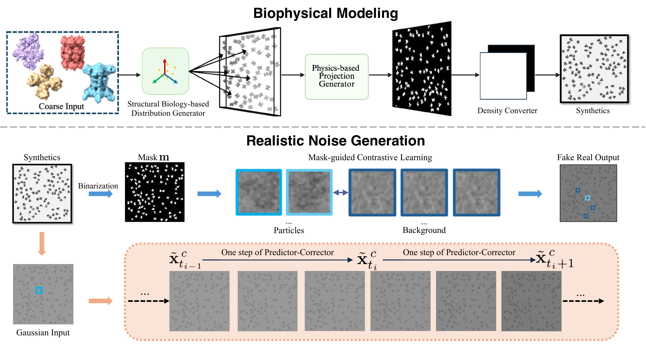
The pipeline has two stages. Biophysical modeling produces clean, fully annotated micrographs with known particle positions, poses and masks; realistic noise generation translates them into the real micrograph domain without paired data.

CryoCCD pipeline: biophysical modeling (top) and realistic noise generation with cycle-consistent predictor–corrector diffusion (bottom).
CryoCCD pipeline. (1) Biophysical modeling: input structures are placed into a 3D volume, then passed through physics-based projection and density conversion. (2) Realistic noise generation: synthetic images are translated into realistic noisy micrographs with cycle-consistent predictor–corrector diffusion and mask-guided contrastive learning. Within one diffusion step, the predictor and corrector advance the state from \(t_{i-1}\) to the corrected state at \(t_i\).

Stage 1 · Biophysical modeling

Structure library

Experimental PDB structures from ~50 kDa enzymes to >50,000 kDa viral capsids, plus AlphaFold3 models that add compositional and conformational heterogeneity.

Particle placement

RELION-derived picks and orientations blended with synthetic samples on \(S^3\); class-specific rules for enzymes, polysomes and capsids.

Multi-scale volume & ice

Scale-adaptive meshes and collision checks; a vitreous ice slab with log-normal thickness and Perlin-noise topography.

Projection & CTF

Summed electrostatic potential, weak-phase projection, and the contrast transfer function applied in Fourier space.

Potential assembly and projection

\[\Phi(\mathbf{r}) = \sum_{i=1}^{L} \rho_i\bigl(R(q_i)^{-1}(\mathbf{r}-T_i)\bigr)\]
\[P(x,y) = \int_{-z_0/2}^{z_0/2} \Phi(x,y,z)\,\mathrm{d}z\]

The electrostatic potential of all \(L\) embedded particles (density \(\rho_i\), orientation \(q_i\), translation \(T_i\)) is projected under the weak-phase approximation; the CTF is then applied in Fourier space.

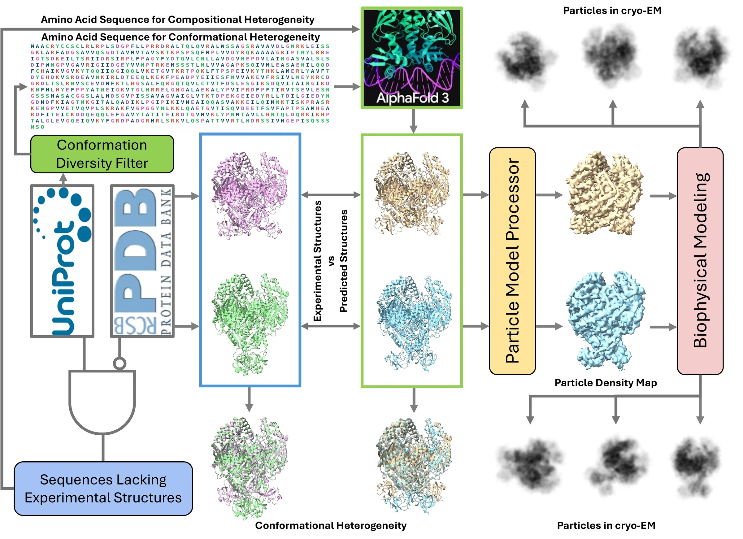
AlphaFold3-based pipeline for enriching the structure library.
AlphaFold3-augmented library. Sequences without experimental structures (UniProt) add compositional heterogeneity; entries with multiple conformations, such as the open and closed states of human PNPase, add conformational heterogeneity.
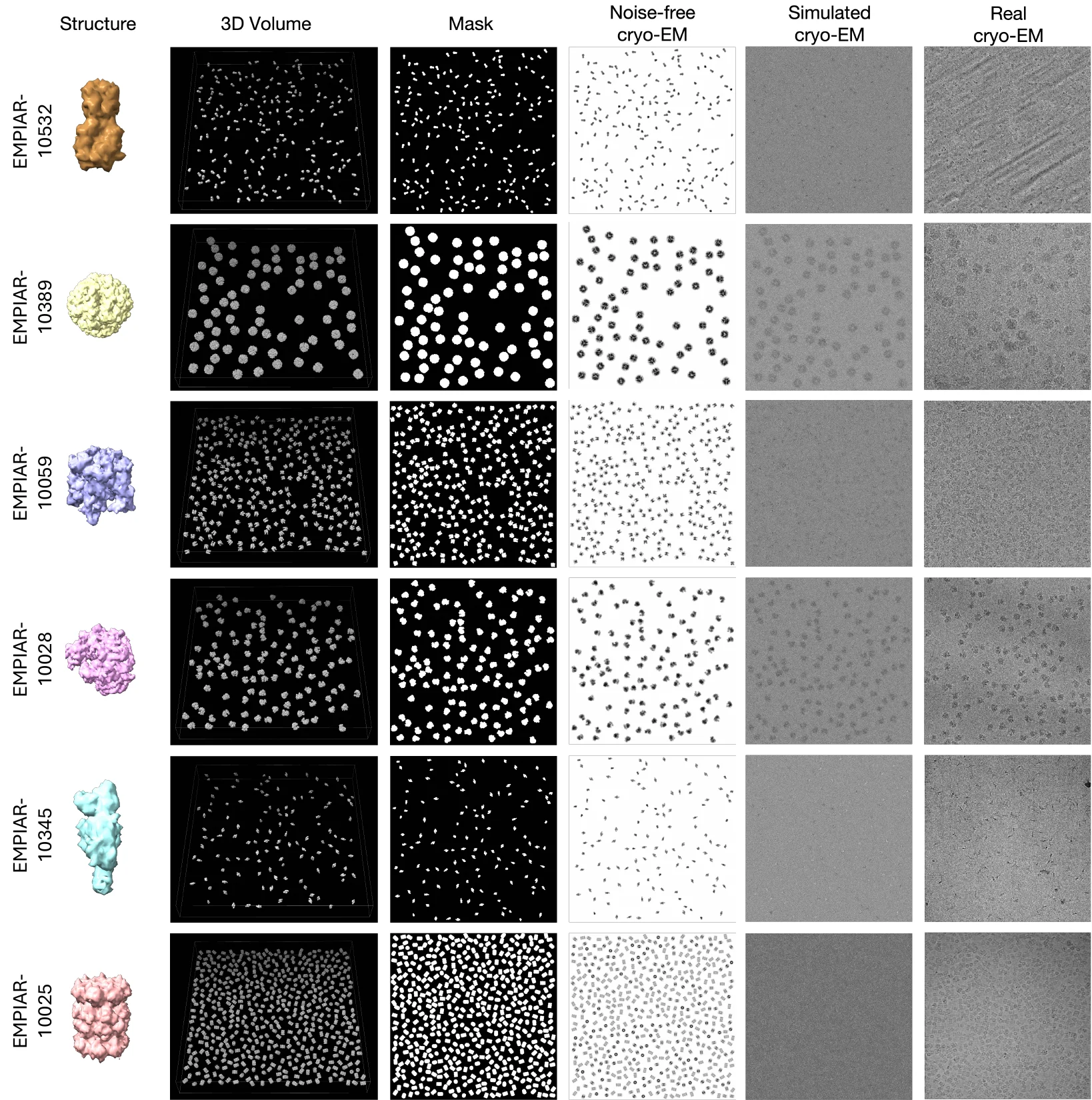
Step-wise visual examples from the CryoCCD simulation pipeline.
Step by step. Structures are embedded into 3D virtual volumes, projected to noise-free micrographs with masks, and then given generated noise; the results sit next to real micrographs.
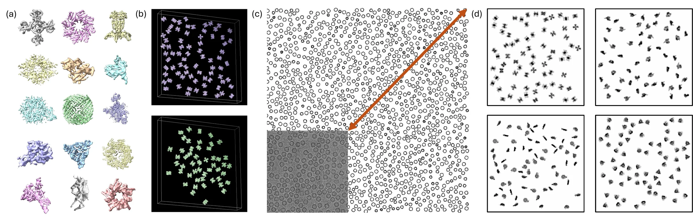
Outputs of the biophysical modeling engine: particle density maps, placement strategies, multi-scale synthesis, and simulated images.
Biophysical modeling outputs. (a) Particle density maps processed from PDB data. (b) Placement strategies chosen by particle properties. (c) Multi-scale synthetic data following EMPIAR-10421. (d) Simulated cryo-EM images.

Stage 2 · Realistic noise generation

Cycle consistency

A mask-conditioned generator \(G_{AB}\) and an unconditional \(G_{BA}\) are tied by an L1 cycle loss in both directions, so particle positions survive translation.

Mask-guided contrastive learning

Segmentation masks define particles as positives and background as negatives, sharpening edges, textures and spatial noise patterns.

Predictor–corrector sampling

A mask-conditioned UniPC sampler in the half log-SNR domain: a \(p\)-th order predictor and a \((p{+}1)\)-th order corrector per step.

Training objective

\[\mathcal{L} = \gamma_{\text{adv}}\mathcal{L}_{\text{adv}} + \gamma_{\text{cyc}}\mathcal{L}_{\text{cyc}} + \gamma_{\text{NCE}}\mathcal{L}_{\text{NCE}}, \qquad \gamma_{\text{adv}}=1,\ \gamma_{\text{cyc}}=3,\ \gamma_{\text{NCE}}=5\]
\[\mathcal{L}_{\text{cyc}} = \mathbb{E}_{(\mathbf{x},\mathbf{m})}\bigl\|G_{BA}(G_{AB}(\mathbf{x},\mathbf{m}))-\mathbf{x}\bigr\|_1 + \mathbb{E}_{\mathbf{y}}\bigl\|G_{AB}(G_{BA}(\mathbf{y}),\varnothing)-\mathbf{y}\bigr\|_1\]
\[\mathcal{L}_{\text{NCE}} = -\log \frac{e^{\cos(q,k^+)/\tau}}{e^{\cos(q,k^+)/\tau} + \sum_{k^-} e^{\cos(q,k^-)/\tau}}\]

The least-squares adversarial term carries the smallest weight; it serves only as an auxiliary distribution-matching regularizer on top of the diffusion sampler.

Results

More realistic micrographs, better downstream models

6 / 6 EMPIAR datasets where CryoCCD has the lowest FID and CMMD
−43% Mean FID vs. the strongest mixed-trained baseline (126.0 vs. 222.1)
0.797 Topaz picking AUPRC on PhageMS2, up from 0.601 for the best baseline
4 / 4 Held-out EMPIAR datasets (unseen families or imaging conditions) won on FID and CMMD

Visual quality

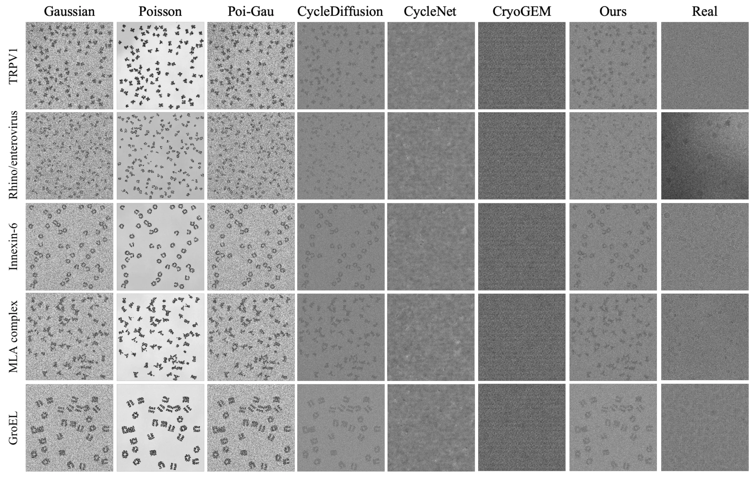
Real micrographs compared with micrographs generated by CryoCCD and baselines across datasets.
Real vs. generated micrographs. CryoCCD reproduces real noise characteristics while preserving particle boundaries and particle–background contrast. Gaussian, Poisson and mixed noise miss the structured noise; CycleDiffusion blurs boundaries; CryoGEM and CycleNet collapse on the composite synthetic data.

FID ↓ / CMMD ↓ on six cryo-EM datasets

MethodTRPV1β-gal.RhinoInnexin-6MLAGroEL
Gaussian
Poisson
Poi–Gau
CycleDiffusion
CryoGEM
CycleNet
CryoCCD (ours)
Separately trained on each dataset (ST)
CryoGEM (ST)
CryoCCD (ST)

Mixed-dataset training unless marked ST. Evaluation micrographs are a disjoint 20% split. CryoCCD also has the lowest radially averaged power-spectrum discrepancy in particle-containing regions on all six datasets (see the appendix).

Downstream: particle picking and pose estimation

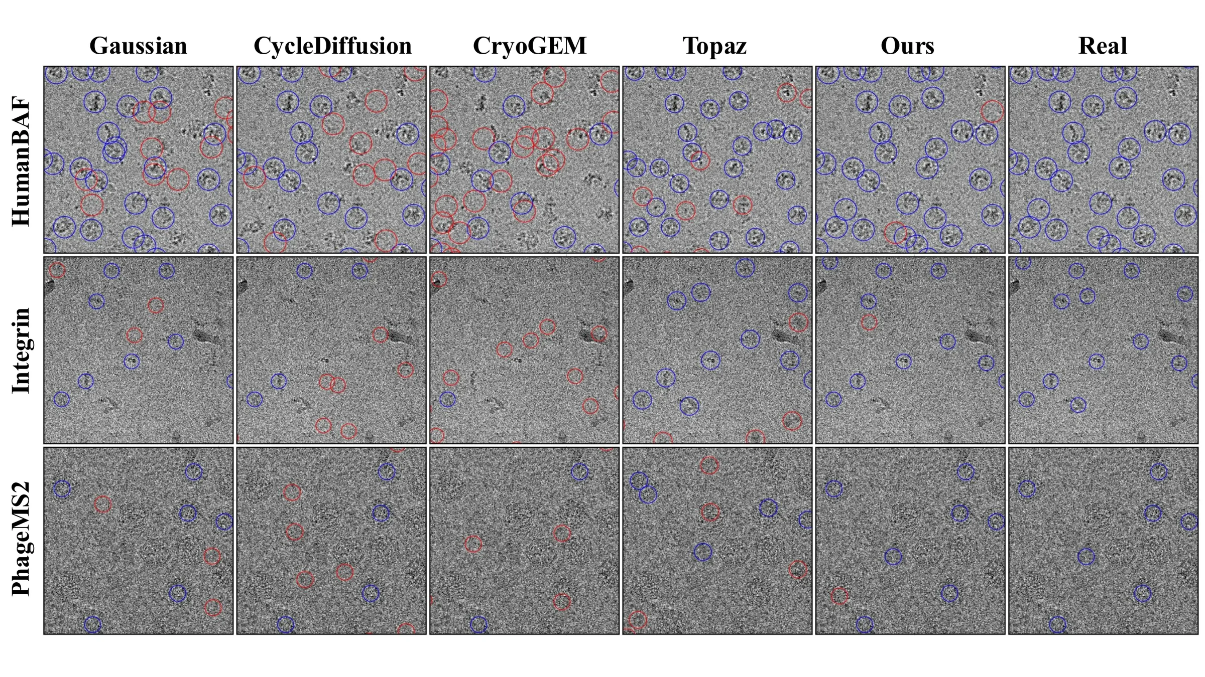
Topaz fine-tuned on CryoCCD micrographs separates particles from background more reliably, and CryoFIRE trained on CryoCCD particles, which come with exact orientation labels, gives lower rotation error and better resolution on real data.

Qualitative comparison of particle picking results across methods.
Particle picking. Blue circles are correct picks; red circles are misses or false picks. Fine-tuning on CryoCCD-generated micrographs gives the highest picking accuracy.

Particle picking · AUPRC ↑

MethodProteasomeIntegrinPhageMS2HumanBAF
Gaussian0.4630.2330.5750.449
Poisson0.4580.1950.4080.392
Poi–Gau0.4380.2440.6010.376
CycleDiffusion0.3570.2330.4200.369
CryoGEM0.2570.2080.1590.178
CycleNet0.3430.2510.3990.297
Topaz0.3010.5100.3170.487
CryoCCD (ours)0.4790.5320.7970.588

Pose estimation · rotation error (rad) ↓

MethodProteasomeIntegrinPhageMS2HumanBAF
Gaussian0.511.490.991.58
Poisson1.091.661.031.60
Poi–Gau1.321.570.731.51
CycleDiffusion0.471.410.971.67
CryoGEM1.721.941.201.78
CycleNet1.031.501.191.69
CryoFIRE1.540.970.751.49
CryoCCD (ours)0.440.900.511.47

Generalization to held-out datasets

FID ↓ on four EMPIAR datasets not used in training

MethodEMPIAR-10028EMPIAR-10059EMPIAR-10389EMPIAR-10532
Gaussian290.34301.07275.46299.01
Poisson443.13389.78391.27410.98
Poi–Gau286.46300.98277.04307.87
CryoGEM232.69247.58244.33280.61
CycleNet210.47227.48230.09222.56
CryoCCD (ours)135.77140.54131.90158.75

EMPIAR-10028, 10389 and 10532 share no protein family with the training data; EMPIAR-10059 (TRPV1) is a held-out imaging condition. CryoCCD also has the lowest CMMD on all four.

Ablation

FID ↓ when removing diffusion or biophysical components

SettingTRPV1β-gal.RhinoInnexin-6MLAGroEL
w/o cycle consistency243.38254.97270.01248.53199.79300.35
w/o mask-guided contrastive155.95163.31159.44169.01122.57191.49
w/o predictor–corrector147.75150.26155.37148.45100.63177.44
Biophysical modeling variants
Global-gradient ice layer199.84270.32212.09228.65197.52284.43
Small-defocus CTF149.33151.79163.31147.28104.01180.43
Large-defocus CTF148.47156.90166.44150.80107.09184.47
Full CryoCCD121.32137.57130.89130.5288.55147.41

Why it matters

Turn a few real annotations into a large synthetic corpus.

Every CryoCCD micrograph comes with exact particle positions, orientations and masks, labels that are slow and error-prone to obtain from real cryo-EM data.

Because the noise is learned from real micrographs rather than assumed to be Gaussian or Poisson, models trained on the synthetic data transfer to real data. CryoCCD can help amplify limited real annotations and speed up the development of computational tools for the cryo-EM community.

Citation

Cite CryoCCD

If you find our work useful in your research, please consider citing:

@article{jiang2026cryoccd,
  title   = {Simulating Cryo-EM: Cycle-Consistent Predictor--Corrector Diffusion with Biophysical Modeling},
  author  = {Runmin Jiang and Genpei Zhang and Yuntian Yang and Siqi Wu and Seonghui Min and Xi Xiao and Yizhou Zhao and Xiao Wang and Tianyang Wang and Xingjian Li and Muyuan Chen and Min Xu},
  journal = {Transactions on Machine Learning Research},
  year    = {2026},
  url     = {https://openreview.net/forum?id=oBBBg2MbGB}
}

Acknowledgement. This work was supported in part by U.S. NSF grant DBI-2238093. We thank Yuheng Zhang for assistance with data analysis.